Statistical Mechanics

Thermodynamics

Thermodynamics, essentially, is a phenomenological description of macroscopic system in thermal equilibrium.

How to idealize the system

View it as some ensemble such as:

• closed system: often descripted as a closed box with adiabatic walls. (Microcanonical)
• open system: with exchanges
  • canonical: exchanges heat. (Two system with diabatic wall)
  • grandcanonical: exchanges both heat and particles, etc.

How to describe the system

• State function
• Thermodynamics coordinates.
• State Variable: \(P\) (Pressure), \(V\) (Volume), \(\mu\) (Chemical Potential), etc.

The idea of SM Thermodynamics(example):

For kinetic theory of gas, the system in micro perspective can be completely described as \[ (\vec p_1,\cdots, \vec p_N, \vec q_1,\cdots, \vec q_N) \] as a point in phase space of dim \(6N\) (3 for 3d).

And in phase space, a probability measure \(P\) is introduced for each state.

The Boltzmann equation and H theorem says that the equilibrium we can observe occurs as the maximization of entropy \(S\)

\[ \begin{aligned} \max&\quad S(P) = \int P \ln P d\omega\\ \text{s.t.}&\quad \int P(\omega) d\omega =1 \quad\text{Probability Measure}\\ &\quad \int \rho(\omega) dP = \chi\quad\text{Energy constraint, etc.}\\ &\quad \text{more constraint } \end{aligned} \]

Use Lagrangrian Multipler: \[ \max \min_{\lambda_1,\lambda_2,\cdots} f(P, \lambda_1,\lambda_2,\cdots) =\int P\ln P d\omega + \lambda_1 \left(\int P(\omega) d\omega -1\right) + \lambda_2 \left( \int \rho(\omega) P d\omega - \chi\right) +\cdots \]

\[ \begin{aligned} &\frac{\delta F}{\delta P} = \ln P +1 + \lambda_1 + \lambda_2\rho(\omega) +\cdots =0 \\ &\Rightarrow P(\omega) = \exp\left(-1-\lambda_1-\lambda_2\rho(\omega)-\cdots\right) \end{aligned} \] Define \[ Z=\int \exp\left(-\lambda_2\rho(\omega)-\cdots\right) d\omega \\ P(\omega) = \frac{\exp\paren{\lambda_2\rho(\omega)-\cdots}}{Z} \] to absorb \(1+\lambda_1\).

Question to be answered:

• Why the equilibrium occurs when \(S\) is maximized (and why \(S\) is in this form?)
• How to calculate the amount we care from this? (To be precise, ensemble averages \(\avg{A}=\int A P d\omega\))

We will go back to this later, but now we shall first look at the classical thermodynamics.

The Zeroth Law of Thermodynamics:

The system is usually of \(10^{20+}\) particles and the possible states are at least of \(\mathcal{O}(\exp(10^{20}))\). How we can use a marco parameter such as temperature to describe a great portion of such possible states?

In common sense, marco parameters are a property shared by physical systems. To make this statement well-defined, we should introduce the zeroth law of Thermodynamics:

(The transitivity of equilibrium) if system A is in equilibrium with system B and system B is in equilibrium with system C. Then A is in equilibrium with system C.

Therefore, a system in thermoequilibrium can be described in a state function that is purely described by its thermocoordinate (things that equals when in thermoequilibrium), as equivalence class in math.

The First Law of Thermodynamics

The amount of work required to change the state of an otherwise adiabatically isolated system depends only on the initial and final states, and not on the means by which the work is performed, or on the intermediate stages through which the system passes.

For the thermodynamics system we can construct a state function, the internal energy \(U(X)\). The amount of \(U\) can be derived from amount of work \(W\) needed for an adiabatic transformation from an inital state \(X_i\) to a final state \(X_f\) using \(\delta W= U(X_i)-U(X_f)\).

What if the transformation is not adiabetic (which is the most of the cases)?

It is observed that \(dU \neq -\delta W\), We call the extra part that cannot be explained by \(\delta W\) as \(\delta Q\)

\[ \delta Q = \delta W + dU \Rightarrow dU = \delta Q -\delta W \]

\[ \text{Measure}\ W_{\text{adiabatic}} \xrightarrow{\text{Define}} U \xrightarrow{\text{Define the difference}} \delta Q \equiv dU + \delta W \]

Sometimes we use generalized force and displacement to charactize the work done:

System	Force	Displacement
Wire	tension \(F\)	length \(L\)
Fluid	pressure \(-P\)	volume \(V\)
Chemical reaction	chemical potential \(\mu\)	particle number \(N\)

Ideal gas: \[ U(T, V) = U(T) \] T does not change during expansion.

Response functions:

Charactizing the macroscopic behaviour of the system:

Heat capacities:

\[ \begin{align} C_V = \frac{\delta Q}{d T}\bigg|_V = \frac{d E + P dV}{d T}\bigg|_V= \frac{\partial E}{\partial T}\bigg|_V\\ C_P = \frac{\delta Q}{d T}\bigg|_P = \frac{d E + P dV}{d T}\bigg|_P= P\frac{\partial V}{\partial T}\bigg|_P + \frac{\partial E}{\partial T}\bigg|_P \end{align} \]

For ideal gas \[ C_P-C_V = P \frac{\partial V}{\partial T}\bigg|_P= Nk_B \]

Isothermal compressibility: \[ \kappa_T \equiv -\frac{1}{V}\frac{\partial V}{\partial P}\bigg|_T \]

The Second Law of Thermodynamics

The impetus for the second law of thermodynamics is the advent of heat engines.

Heat engine: a device that receives energy in the form of heat from a hot reservoir, delivers work to its surroundings, and discharges energy in the form of heat to a cold reservoir.

Heat pump: a device that uses work to delivers energy in the form of heat to a hot reservoir, and receives energy in the form of heat from a cold reservoir.

-------                      ------
|Source|--Qh->|Engine|--Q_c->|Sink|
-------         |            ------
                |
                v
               Work

               Work
                |
                |
                v
-------                       -------
|Icebox|--Qc->|Fridge| --Qh->|Exhaust|
-------                       ------- 

\[ Q_h = W + Q_c \] Heat engine efficiency: \[ \eta = \frac{W}{Q_h} = 1 - \frac{Q_c}{Q_h} \leq 1 \]

Heat pump efficiency: \[ \eta = \frac{Q_c}{W} \]

The second law of thermodynamics states that the efficiency of a heat engine can never be 100%.

Kelvin’s Statement: No process is possible whose sole result is the complete conversion of heat into work.

Clausius’s Statement: No process is possible whose sole result is the transfer of heat from a cooler to a hotter body.

The best heat engine is the Carnot engine, which consists of two isothermal processes and two adiabatic processes.

1. Isothermal expansion: the system is in contact with the hot reservoir at temperature \(T_h\), and expands from volume \(V_1\) to \(V_2\).
2. Adiabatic expansion: the system is isolated and expands from volume \(V_2\) to \(V_3\).
3. Isothermal compression: the system is in contact with the cold reservoir at temperature \(T_c\), and compresses from volume \(V_3\) to \(V_4\).
4. Adiabatic compression: the system is isolated and compresses from volume \(V_4\) to \(V_1\).

See https://galileo.phys.virginia.edu/classes/152.mf1i.spring02/CarnotEngine.htm for more details.

We argue that the efficiency of the Carnot engine is the upper bound of all heat engines, otherwise we can use the more efficient engine to run the Carnot engine in reverse to create a perpetual motion machine of the second kind (Pump heat from cold to hot without work input).

Use the ideal gas as an example, we can calculate the efficiency of the Carnot engine is \[ \eta = 1 - \frac{T_c}{T_h} \]

And the result is irrelevant to the working substance by the fact that the efficiency of the Carnot engine is most efficient.

Therefore, the efficiency of any heat engine is bounded by the efficiency of the Carnot engine: \[ \frac{\delta W}{\delta Q} \leq 1 - \frac{T_c}{T_h} \]

The Third Law of Thermodynamics

For an infinismal process that draw \(\delta Q\) from a heat reservoir at temperature \(T_h\)

W.r.t. the whole system: \[ \oint dU =0 \Rightarrow \oint \delta Q = \oint \delta W \]

We can decompose any process into a series of infinitismal processes, and for each process, the system exchange heats with a system with almost identical temperature. We know that: \[ \delta W_i \leq \left(1 - \frac{T_c}{T_i}\right) \delta Q_i \] where \(T_i\) is the temperature of the system during the \(i\)-th process. Therefore, we have: \[ \begin{gather*} \sum_{i=1}^\infty \delta W_i \leq \sum_{i=1}^\infty \left(1 - \frac{T_c}{T_i}\right) \delta Q_i \leq \sum_{i=1}^\infty \delta Q_i - \frac{T_c}{T_i} \delta Q_i = \sum_{i=1}^\infty \delta Q_i - T_c \sum_{i=1}^\infty \frac{\delta Q_i}{T_i} \\ T_c \sum_{i=1}^\infty \frac{\delta Q_i}{T_i} \leq 0 \end{gather*} \]

Which leads to Clausius’s theorem \[ \oint \frac{\delta Q}{T} \leq 0 \]

For a reversible cycle, we infer that \(\frac{\delta Q}{T}=0\). And we can define a function of state \(S\), only dependent on two end-points: \[ S(A)-S(B) = \int_B^A \frac{dQ_{rev}}{T} \]

Kinetic Theory of Gas

Liouville Theorem

\[ q'=q+\dot q \delta t + O(\delta t^2), p'=p+\dot p \delta t + O(\delta t^2), \] \[ dq'=dq+\partial_q \dot q\ dq \delta t + O(\delta t^2), dp'=dp+\partial_p \dot p\ dp \delta t + O(\delta t^2) \]

\[ d \Gamma' = \prod_{\alpha=1}^{3N} dq'_{\alpha} dp'_{\alpha} = \prod_{\alpha=1}^{3N} (1+(\partial_q \dot q+\partial_p \dot p )\delta t + O(\delta t^2))dq_{\alpha} dp_{\alpha} \] Since \(\partial_q \dot q+\partial_p \dot p=\partial_{qp} H -\partial_{pq} H =0\). \[ d\Gamma = d \Gamma' \] So \(\frac{d\rho}{dt}=0\).

\[ \begin{align} \frac{d\rho}{dt} &= \partial_t \rho + \sum_\alpha \left(\dot{q}_\alpha\,\partial_{q_\alpha}\rho + \dot{p}_\alpha\,\partial_{p_\alpha}\rho\right) = 0\\ \partial_t \rho &= -\{\rho, \mathcal{H}\} \end{align} \] \[ \{\rho,\mathcal{H}\} = \partial_{p_{\alpha}} \mathcal{H}\partial_{q_\alpha}\rho-\partial_{q_\alpha}\mathcal{H}\partial_{p_{\alpha}}\rho \] The time evolution of the ensemble average \[ \begin{aligned} \frac{d\langle O\rangle }{dt} &= \frac{d}{dt}\int O(p,q,t) \rho(p,q,t) d\Gamma\\ &=\int\frac{dO}{dt}\rho+\underbrace{O\frac{d\rho}{dt}}_{0} d\Gamma \\ &=\left\langle\frac{dO}{dt}\right\rangle \\ &=\langle \{O,H\}\rangle \quad \text{If O is not explicitly depend on time} \end{aligned} \]

Now, consider the equilibrium state: \[ \partial_t \rho = -\{\rho, H\} =0 \] A possible solution is \[ \rho = \rho(\mathcal{H}(p,q)) \] constant on constant energy surface, etc. or \(\rho =\rho(H,L,\cdots)\) for additional conserved quantities.

non-stationary densities converge onto the stationary solution

Actually, this is the fact that the solutions are in the neighborhood of \(\rho_{eq}\) for the most of the time.

Need ergodicity to justify.

BBGKY Hierarchy

Define s-partial density \[ f_s(p_1,q_1,\cdots,p_s,q_s) = \frac{N!}{(N-s)!}\int\prod_{i=s+1}^N dV_i\rho(p_1,q_1,\cdots,p_N,q_N,t)= \frac{N!}{(N-s)!}\rho_s(p_1,q_1,\cdots,p_s,q_s,t) \] Assume the Hamiltonian \[ \begin{aligned} \mathcal{H}(p,q)&=\sum_{i=1}^N\left[\frac{p_i^2}{2m}+U(q_i)\right]+\frac{1}{2}\sum_{(i,j)=1}^N\mathcal{V}(q_i-q_j)\\ &=\sum_{i=1}^s\left[\frac{p_i^2}{2m}+U(q_i)\right]+\frac{1}{2}\sum_{(i,j)=1}^s \mathcal{V}(q_i-q_j)\\ &\ +\sum_{i=s+1}^{n}\left[\frac{p_i^2}{2m}+U(q_i)\right]+\frac{1}{2}\sum_{(i,j)=s+1}^N\mathcal{V}(q_i-q_j)\\ &\ + \sum_{i=1}^s\sum_{j=s+1}^N \mathcal{V}(q_i-q_j)\\ &=\mathcal{H}_s+\mathcal{H}_{n-s}+\mathcal{H}'\\ \end{aligned} \] \[ \partial_t \rho_s = -\int \prod_{i=s+1}^N dV_i\{\rho,\mathcal{H}\} = -\underbrace{\int \prod_{i=s+1}^N dV_i \{\rho,\mathcal{H}_{s}\}}_{\{\rho_s,\mathcal{H_s}\}} - \underbrace{\int \prod_{i=s+1}^N dV_i\{\rho,\mathcal{H}_{n-s}\}}_{0}-\int \prod_{i=s+1}^N dV_i\{\rho,\mathcal{H'}\} \]

\[ \begin{aligned} -\int \prod_{i=s+1}^N dV_i \{\rho,\mathcal{H}'\} &= -\int \prod_{i=s+1}^N dV_i \left(\underbrace{\sum_{j=1}^N\partial_{p_j}{\mathcal{H}'}\partial_{q_j} \rho}_{0}-\partial_{q_j} \mathcal{H}' \partial_{p_j} \rho\right) \\ &= \int\prod_{i=s+1}^N d V_i \left(\sum_{j=1}^N \partial_{q_j}\mathcal H' \partial_{p_j} \rho\right)\\ &= \int\prod_{i=s+1}^N d V_i \left(\sum_{j=1}^N \partial_{p_j} (\rho \partial_{q_j}\mathcal H')\right) \quad \text{since } \partial_{p_j} \mathcal{H'}=0\\ &= \int\prod_{i=s+1}^N d V_i \left(\sum_{j=1}^s \partial_{p_j} (\rho \partial_{q_j}\mathcal H')\right)\\ &= \int\prod_{i=s+1}^N d V_i \left(\sum_{j=1}^s \partial_{p_j} \rho \partial_{q_j}\mathcal H'\right)\\ &= \int\prod_{i=s+1}^N d V_i \left(\sum_{j=1}^s \partial_{p_j} \rho\sum_{n=s+1}^N \partial_{q_j} \mathcal{V}(q_j-q_n)\right)\\ &= (N-s)\sum_{j=1}^s \int dV_{s+1}\, \frac{\partial \mathcal{V}(q_j - q_{s+1})}{\partial q_j}\cdot \frac{\partial}{\partial p_j}\underbrace{\int \prod_{i=s+2}^N dV_i\, \rho}_{\rho_{s+1}}\\ &= (N-s)\sum_{j=1}^s \int dV_{s+1}\, \frac{\partial \mathcal{V}(q_j - q_{s+1})}{\partial q_j}\cdot \frac{\partial \rho_{s+1}}{\partial p_j} \end{aligned} \]

BBGKY Formula

\[ \partial_t \rho_s - \{\mathcal H_s,\rho_s\} = (N-s)\sum_{j=1}^s \int dV_{s+1}\, \frac{\partial \mathcal{V}(q_j - q_{s+1})}{\partial q_j}\cdot \frac{\partial \rho_{s+1}}{\partial p_j} \] or \[ \partial_t f_s - \{\mathcal H_s,f_s\} = \sum_{j=1}^s \int dV_{s+1}\, \frac{\partial \mathcal{V}(q_j - q_{s+1})}{\partial q_j}\cdot \frac{\partial f_{s+1}}{\partial p_j} \] Note that the LHS is the full time derivative of \(\rho_s\), or action under \[ D_t = (\partial_t+\dot q_{\alpha}\partial_{q_\alpha}+\dot p_{\alpha}\partial_{p_\alpha}) \] adjusted by a scatter term (RHS).

---

Boltzmann Equation & H-Theorem

First Level in BBGKY equation \(\dot q= \partial_{p} H = \frac{p}{m}\) \(\dot p=-\partial_q H = \partial_q V\) \[ \begin{gather} \left[\partial_t + \frac{p_1}{m} \partial_{q_1} - \partial_{q_1} U \partial_{p_1}\right] f_1 = \int dV_{2} \partial_{q_1} \mathcal{V}(q_1-q_2) \partial_{p_1} f_2\\ \left[\partial_t + \frac{p_1}{m}\partial_{q_1} + \frac{p_2}{m}\partial_{q_2}-\partial_{q_1} U \partial_{p_1} - \partial_{q_2} U \partial_{p_2} - \partial_{q_1} \mathcal{V}(q_1-q_2) [\partial_{p_1}-\partial_{p_2}]\right] f_2 = \\ \int dV_3 \left[\partial_{q_1}\mathcal{V}(q_1-q_3)\partial_{p_1}+\partial_{q_2}\mathcal{V}(q_2-q_3)\partial_{p_2}\right]f_3 \end{gather} \]

Estimation \[ \begin{gather} v\sim 10^2\text{ m/s}\\ \tau_{coll} \approx r_0 / v\\ \frac{1}{\tau_c} \sim \partial_q{\mathcal V}\partial_p \sim \frac{v}{d=10^{-10}\text{m}}\approx 10^{12}s^{-1}\\ \frac{1}{\tau_U} \sim \partial_q{U}\partial_p \sim \frac{v}{L=10^{-3}\text{m}}\approx 10^{5}s^{-1}\\ \frac{1}{\tau_x} \sim \frac{nd^3}{\tau_c} \approx 10^{8} s^{-1} \end{gather} \]

LHS of \((1) \sim \frac 1{\tau_U}\) RHS of \((1) \sim \frac{1}{\tau_x}\) LHS of \((2) \sim \frac{1}{\tau_\text{coll}}\) RHS of \((2) \sim \frac{1}{\tau_x}\)

So we can set RHS of \((2)\) to 0.

\[ \begin{gather} \left[\partial_t + \frac{p_1}{m} \partial_{q_1} - \partial_{q_1} U \partial_{p_1}\right] f_1 = \int dV_{2} \partial_{q_1} \mathcal{V}(q_1-q_2) \partial_{p_1} f_2\\ \left[\partial_t + \frac{p_1}{m}\partial_{q_1} + \frac{p_2}{m}\partial_{q_2}-\partial_{q_1} U \partial_{p_1} - \partial_{q_2} U \partial_{p_2} - \partial_{q_1} \mathcal{V}(q_1-q_2) [\partial_{p_1}-\partial_{p_2}]\right] f_2 = 0 \end{gather} \]

\[ L f_2 =\frac{df_2}{dt}=0 \] And assume when \(q_1, q_2\) distant \[ f_2(p_1,q_1,p_2,q_2,t) \xrightarrow{|q_1-q_2| \gg d} f_1(p_1,q_1,t) f_2(p_2,q_2,t)\quad \text{Molecular Chaos} \] So \[ f_2(q_1, p_1, q_2, p_2, t) = f_1(q_1, p_1^{(-\infty)}, t) f_1(q_2, p_2^{(-\infty)}, t) \] \(q_1(-\infty) \approx q_1\) since the position won’t change so much.

\[ \begin{gather} \left[\partial_t + \frac{p_1}{m}\partial_{q_1} + \frac{p_2}{m}\partial_{q_2}-\partial_{q_1} U \partial_{p_1} - \partial_{q_2} U \partial_{p_2} \right] f_2 = \partial_{q_1} \mathcal{V}(q_1-q_2) [\partial_{p_1}-\partial_{p_2}] f_2 \\ \int dV_2 \partial_{q_1}\mathcal{V}(q_1-q_2)\partial_{p_2}f_2 = \int d q_2 \partial_{q_1}\mathcal{V}(q_1-q_2) \underbrace{\int d p_2 \partial_{p_2}f_2}_{0} =0 \end{gather} \] Therefore, substitute into RHS of \((1)\):

\[ \begin{aligned} \left[\partial_t + \frac{p_1}{m} \partial_{q_1} - \partial_{q_1} U \partial_{p_1}\right] f_1 &= \int dV_2 \left[\partial_t + \frac{p_1}{m}\partial_{q_1} + \frac{p_2}{m}\partial_{q_2}-\partial_{q_1} U \partial_{p_1} - \partial_{q_2} U \partial_{p_2} \right] f_2 \\ \end{aligned} \]

Change variable with \(r = q_1-q_2, R= \frac{q_1+q_2}{2}\) , \(P=p_1+p_2\), \(p=p_1-p_2\).

\[ \mathrm{RHS} \approx \int dp d^3r \frac{p}{m} \partial_r f_2 \] Since \(U\) term and \(\partial_t\) term is small, \(r\) now be the coord along the line.

coll_illustration

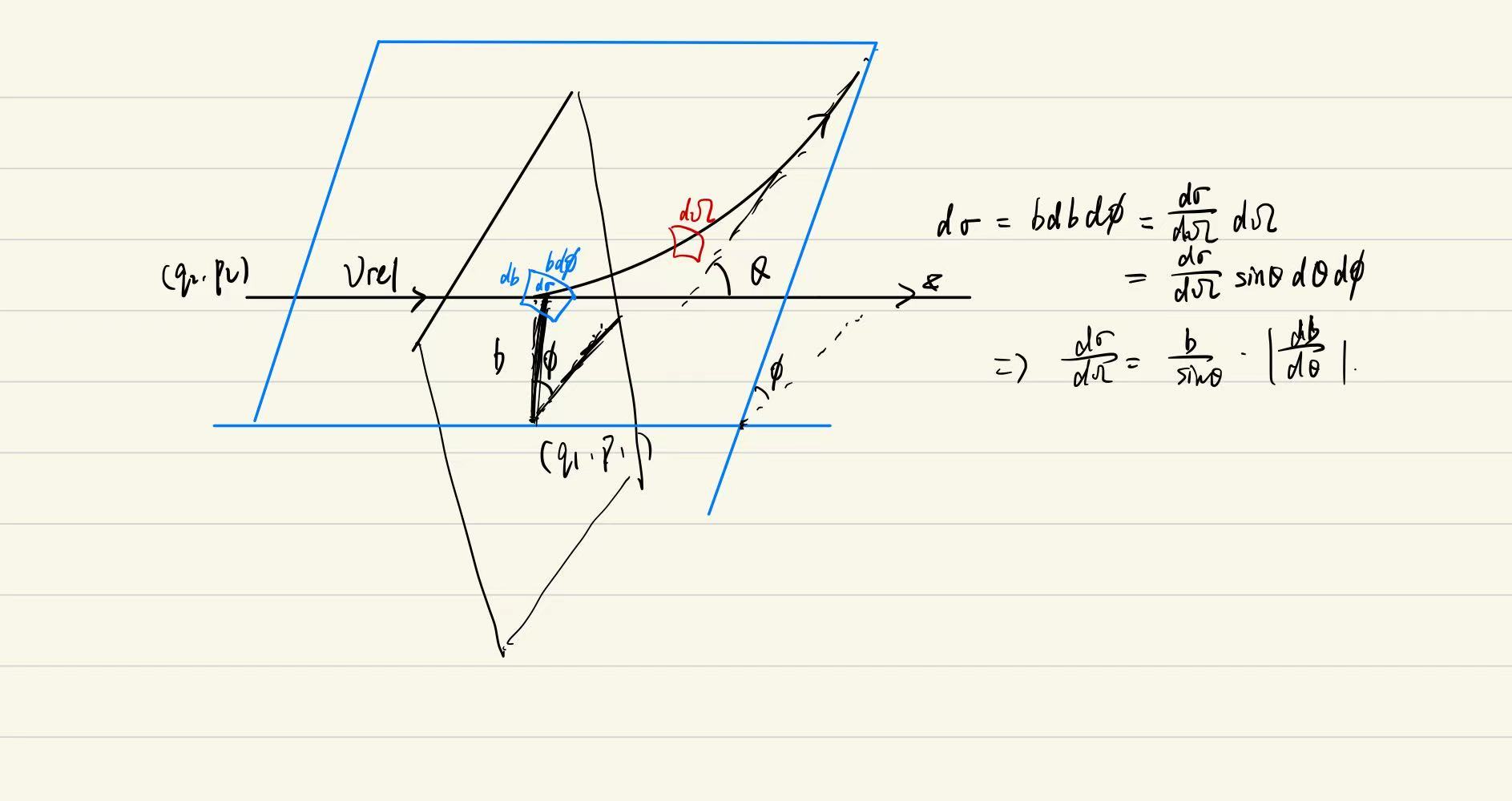
\[ \begin{align} &= \int dp d^2b dr \frac{|p|}{m} \partial_r f_2 \\ &= \int dp d^2b \frac{|p|}{m} \left[f_1(p_1')f_1(p_2')-f_1(p_1)f_1(p_2)\right] \\ &= \int dp b db d\phi \frac{|p|}{m} \left[f_1(p_1')f_1(p_2')-f_1(p_1)f_1(p_2)\right] \\ &= \int \frac{|p_1-p_2|}{m}dp \frac{d\sigma}{d \Omega}d\Omega \left[f_1(p_1')f_1(p_2')-f_1(p_1)f_1(p_2)\right] \\ \end{align} \] We conclude that \[ \frac{d f_1(q(t),p(t),t)}{dt}=\int \frac{p}{m}dp \frac{d\sigma}{d \Omega}d\Omega \left[f_1(p_1')f_1(p_2')-f_1(p_1)f_1(p_2)\right] \\ \]

H Theorem

\[ H=\int d^3pd^3q f_1(p,q,t)\ln f_1(p,q,t) \]

\[ \frac{d H}{dt}= \int \frac{1}{m} dp \frac{d\sigma}{d\Omega} d\Omega \left[f_1(p_1')f_1(p_2')-f_1(p_1)f_1(p_2)\right]\ln f_1(p_1) \]

By the Livouille Theorem, we can swap \(p_1'\) and \(p_1\), \(p_2'\) and \(p_2\). By the symmetricity of \(p_1, p_2\), we can swap the subscript too.

\[ \frac{d H}{dt}= \int \frac{1}{4m} dp \frac{d\sigma}{d\Omega} d\Omega \left[f_1(p_1')f_1(p_2')-f_1(p_1)f_1(p_2)\right][\ln f_1(p_1)f_1(p_2)-\ln f_1(p_1') f_1(p_2')] \leq 0 \]

\[ S_{thermo} = -k_B H \]

Equilibrium properties

\[ \frac{dH}{dt} = 0 \] A necessary condition for \(\frac{dH}{dt}=0\) is that \[ f_1(\vec p_1, \vec q_1) f_1(\vec p_2, \vec q_2) = f_1(\vec p_1', \vec q_1) f_1(\vec p_2', \vec q_2) \] at each point \(\vec q\) \[ \ln f_1(\vec p_1, \vec q_1)+\ln f_1(\vec p_2, \vec q_2) = \ln f_1(\vec p_1', \vec q_1)+\ln f_1(\vec p_2', \vec q_2) \] We observed additive conserved quantities in the collision.

1. Number of particles
2. Momentum
3. Energy \[ \ln f_1 = a(q)-\alpha(q)\cdot p -\beta(q)\left(\frac{p^2}{2m}\right) \] Or with potential energy \[ \ln f_1 = a(q)-\alpha(q)\cdot p -\beta(q)\left(\frac{p^2}{2m} + U(q)\right) \] \[ \begin{aligned} f_1 = \mathcal{N}(q) \exp\left(\alpha(q)\cdot p -\beta(q) \left(\frac{p^2}{2m}\right)\right) \end{aligned} \] Assume uniform, \(\{\mathcal H,f_1\}=0\) , \(f_1\) only depend on \(H_1\) or any other quantity that is conserved by it . For example, as long as \(N\), \(\beta\) independent of \(q\) and \(\alpha=0\).

\[ N=\mathcal N V\int \exp\left(- \alpha(q)\cdot p -\beta(q)\left(\frac{p^2}{2m}\right)\right) d^3p = \mathcal{N} V\left(\frac{2m\pi}{\beta}\right)^{\frac {3}{2}}\exp\left(\frac{m\alpha ^2}{2\beta}\right) \] \[ \begin{aligned} \mathcal N &= \frac{N}{V} \left(\frac{\beta}{2m\pi}\right)^{\frac {3}{2}}\exp\left(-\frac{m\alpha ^2}{2\beta}\right) \\ f_1 &= n \left(\frac{\beta}{2m\pi}\right)^{\frac {3}{2}} \exp\left(-\frac{(p-p_0)^2}{2\frac{m}{\beta}}\right)\\ p_0 &= \frac{m\alpha}{\beta}, n=\frac{N}{V} \end{aligned} \] \[ \avg {p^2} = \frac{3m}{\beta} \] Assume \(\alpha=0\).

Equilibrium between two gases:

\[ \begin{gather} C_{a,b}=-\int d^3 p_2 d^2 \Omega \left|\frac{d\sigma_{a,b}}{d\Omega}\right| |v_1-v_2| \left[f_1^{a}(p_1,q_1)f_1^{b}(p_2,q_1) - f_1^{a}(p_1',q_1)f_1^{b}(p_2',q_1)\right]\\ \begin{cases} \partial_t f_1^{(a)} =\{\mathcal{H}_1^{(a)},f_1^{(a)}\} + C_{a,a}+C_{a,b}\\ \partial_t f_1^{(b)} =\{\mathcal{H}_1^{(b)},f_1^{(b)}\} + C_{b,b}+C_{b,a}\\ \end{cases} \end{gather} \]

Equilibrium, all right assume to be zero.

\[ \begin{gather} C_{a,a}=0\Rightarrow f_1^{(a)} \propto \exp(-\beta_a\mathcal H_{1}^{(a)})\\ C_{b,b}=0\Rightarrow f_1^{(b)} \propto \exp(-\beta_b\mathcal H_{1}^{(b)})\\ C_{a,b}=0\Rightarrow f_1^{(a)}(p_1)f_1^{(b)}(p_2)=f_1^{(a)}(p_1')f_1^{(b)}(p_2')\\ \Rightarrow \beta_a \mathcal{H}_1^{(a)}(p_1)+\beta_b\mathcal{H}_1^{(b)}(p_2) = \beta_a \mathcal{H}_1^{(a)}(p_1')+\beta_b\mathcal{H}_1^{(b)}(p_2') \end{gather} \] Can be satisfied with \[ \beta_a=\beta_b=\beta \] \[ \avg{\frac{\vec p_a^2}{2m}} = \avg{\frac{\vec p_b^2}{2m}} =\frac{3}{2\beta} \] Ideal Gas Equation

\[ \begin{gather} d\mathcal{N}(p)=f_1(p)d^3p (Av_x\delta t)\\ F = \frac{1}{\delta t} \iint_{-\infty}^{\infty} \int_0^{\infty} f_1(p) \left(A\frac{p_x}{m}\delta t\right) 2p_x dp_x d p_ydp_z\\ P = F/A = \int d^3 p f_1(p)\frac{p_x^2}{m} = \avg{\frac{p_x^2}{m}} = \frac{n}{\beta} \end{gather} \]

Conservation Law

Stage 1:

Governed by the fast collision term in the right of Boltzmann equation. (reached zero) equilibrium.

local density, governed by the local conservatives.

\[ \begin{aligned} n(q,t)=\int d^3p f_1(p,q,t)\\ \avg{O(q,t)} = \frac{1}{n(q,t)} \int d^3 p f_1 O(p,q,t) \end{aligned} \]

Stage 2:

Governed by the streaming term

It is most conveniently expressed in terms of the time evolution of conserved quantities according to hydrodynamic equations.

Conserved quantity \(\chi\)

\(\chi(p_1,q,t) +\chi (p_2,q,t) = \chi(p'_1,q,t) + \chi(p'_2,q,t)\)

\[ J_{\chi}(q,t) = \int d^3 p \chi(p,q,t) \frac{df_1}{dt}\bigg|_{coll} (p,q,t) =0 \]

If conserved in collision \(\Rightarrow\) does not change.

Now for the left term: \[ \int d^3p\,\chi \left[\partial_t + \frac{p}{m}\cdot\partial_q+ F\cdot\partial_p \right]f_1 = \underbrace{\int d^3p\,\chi\frac{df_1}{dt}\bigg|_\text{coll}}_{=0} \] \[ \begin{gather} \int d^3 p \left[\partial_t + \frac{p}{m}\cdot\partial_q+ F\cdot\partial_p \right](\chi f_1) - f_1 \left[\partial_t + \frac{p}{m}\cdot\partial_q+ F\cdot\partial_p \right]\chi =0 \\ \iff n\partial_t \avg{\chi} +\partial_{q_{\alpha}}\left(n\avg{\frac{p_{\alpha}}{m}\chi}\right) - n\avg{\partial_t \chi} - n\avg{\frac{p_{\alpha}}{m}\partial_{q_{\alpha}}\chi}-nF_{\alpha}\cdot \avg{\partial_{p_{\alpha}}\chi} =0 \end{gather} \] Particle Number (\(\chi=1\)) \[ \partial_t \avg{n} + \partial_{q_{\alpha}}\left(nu_{\alpha}\right) = 0, u=\avg{\frac{p}{m}} \]

Momentum (\(c\equiv\frac{p}{m}-u\))

\[ \begin{gather} n\underbrace{\partial_t\avg{c}}_{0}+\underbrace{\partial_{q_{\alpha}}\paren{n\avg{(c_{\alpha}+u)c}}}_{n\p_{q_{\alpha}}\avg{c_\alpha c_\beta}}-n\underbrace{\avg{\p_t c}}_{-\partial_t u}-n\underbrace{\avg{\frac{p_\alpha}{m}\p_{q_{\alpha}}c}}_{-nu_\alpha\partial_{q_\alpha}u_\beta}-nF_{\alpha}\cdot \underbrace{\avg{\p_{p_\alpha}c}}_{\frac{1}{m}}=0\\ \partial_t u_\alpha + u_\beta\partial_{q_\beta}u_\alpha = \frac{F_\alpha}{m} - \frac{1}{mn} \partial_{q_\beta}(P_{\alpha\beta})\\ P_{\alpha\beta} = mn\langle c_\alpha c_\beta\rangle \end{gather} \]

If \(P_{\alpha\beta} = P\delta_{\alpha\beta}\): \[ \boxed{mn\left(\partial_t u_\alpha + u_\beta\partial_{q_\beta}u_\alpha\right) = nF_\alpha - \partial_{q_\beta}P_{\alpha\beta}} \] Kinetic Energy

Plug in the peculiar speed

\[\vareps\equiv\avg{mc^2/2} = \avg{p^2/2m - p\cdot u+ mu^2/2}\]

\[ \begin{align} &n\p_t \avg {\vareps} + \p_{q_\alpha} \paren{n\avg{\frac{p_\alpha}{m}\vareps}} - n \avg{\p_t \vareps} - n \avg{\frac{p_\alpha}{m}\p_{q_\alpha}\vareps} - nF_{\alpha}\cdot \avg{\p_{p_\alpha}\vareps}=0\\ & \end{align} \] \[ \begin{align} \langle \vareps \rangle &= \avg{\frac{p^2}{2m}}- mu^2 + \frac{mu^2}{2} = \avg{\frac{p^2}{2m}} - \frac{1}{2}mu^2\\ \p_t \avg{\vareps} &=\partial_t \avg{\frac{p^2}{2m}} -mu\cdot \p_t u \end{align} \]

Zeroth-Order Solution

Assume \(f_1\) is in local equilibrium:

\[f_1^{(0)}(\vec{p},\vec{q},t) = \frac{n(\vec{q},t)}{\left(2\pi mk_BT(\vec{q},t)\right)^{3/2}} \exp\left(-\frac{(\vec{p}-m\vec{u})^2}{2mk_BT(\vec{q},t)}\right)\]

This satisfies the collision term exactly (RHS of Boltzmann = 0), but does not satisfy the full Boltzmann equation because the streaming operator \(\mathcal{L}\) acts on the slowly varying fields \(n, \vec{u}, T\).

First order equation

\[ \begin{gather} f_1=f^0(1+g)\\ \frac{df_1}{dt}\bigg|_\text{coll} \approx -\frac{f_1 - f^{(0)}}{\tau} = -\frac{f^{(0)}g}{\tau}\\ \hat{L}f^{(0)} = -\frac{f^{(0)}g}{\tau}\\ g = -\tau \frac{\hat{L}f^{(0)}}{f^{(0)}} \end{gather} \]

(Classical) Statistical Mechanics

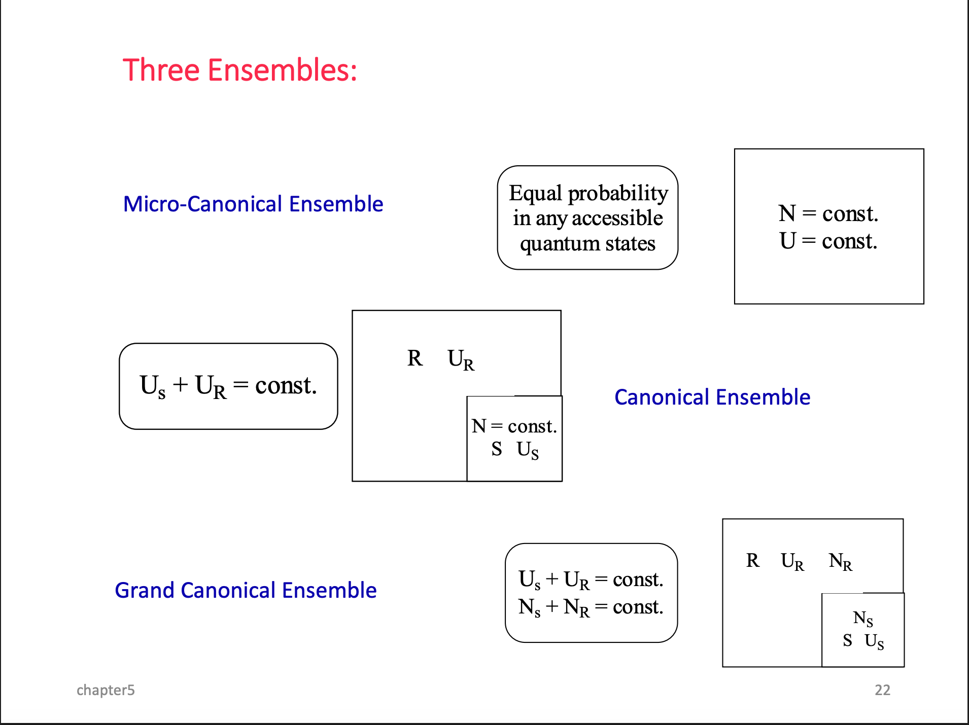
The idea is that we start from the simplest situation (microcanonical). Then we gradually allow extensive quantity to fluctuate but add intensive quantity in control.

Microcanonical System

Particles system where \((E, V, N)\) is fixed.

The system is equally probable in any state that satisfy the energy constraint.

\[ P(\rho) =\begin{cases} \frac{1}{\Omega}\quad U(\rho) =E \\ 0 \quad \text{otherwise} \end{cases} \]

\[ \propto 1 \quad \text{Equally weighted} \]

Canonical System

We now fix \(T\) instead of \(E\) for a system in contact with a heat reservoir.

Consider the whole system \(R\otimes S\), where \(R\) is the heat reservior, \(S\) is the canonical system we want to study.

For the whole system \(R\otimes S\), it is in the microcanonical ensemble.

\[ \begin{aligned} P(\sigma_R, \sigma_S) &\propto \delta(H_R(\sigma_R)+H_S(\sigma_S)-E)\\ P(\sigma_S) &\propto \int d\sigma_R \delta(H_R(\sigma_R)+H_S(\sigma_S)-E)\\ &= \int d\sigma_R \delta(H_R(\sigma_R)-E+H_S(\sigma_S))\\ &= \Omega_R(E-H_S(\sigma_S))\\ &\approx \Omega_R(E) \exp\left(-\beta H_S(\sigma_S)\right) \end{aligned} \]

The last step is expand \(\ln \Omega_R\) at \(E\) to the first order, and use \(\beta = \frac{\partial \ln \Omega_R}{\partial E}\).

Question:

Why not expand \(\Omega_R\) directly? Hint: \(\Omega_R\) is exponential in \(E\). Draw \(\exp x\)’s expansion at \(x=100\) to see the difference.

Grandcanonical System

We now fix \(\mu\) instead of \(N\), allowing particle number to fluctuate.

For similar reason, the system can be in energy \(E\), particle number \(N\) with probability: \[ \propto \exp(-\beta (E -\mu N)) \]

Gibbs System

Fix \((T,P,N)\), change \(V\) to \(P\), \(E\) to \(T\).

\[ \propto \exp(-\beta(E+PV)) \]

Partition Function and the Calculations

Here we assume the hamiltonian is \[ H = \sum_{i=1}^N \frac{p_i^2}{2m} \] \(N\) non-interacting particles in a box of volume \(V\) and potential energy \(U=0\).

\[ Z = \int d \omega p(\omega) \] where \(p(\omega)\) is unnormalized distribution.

In microcanonical ensemble:

\[ \begin{aligned} \Omega(E) &= \frac{1}{h^{3N} N!}\int d \omega \delta(H(\omega ) -E) \\ &= \frac{1}{h^{3N} N!}\int \prod_{i=1}^N d^{3}q_i d^{3} p_i \delta \left(\sum_{i=1}^N \frac{p_i^2}{2m} - E\right) \\ &= \frac{V^{N}}{h^{3N} N!} \int \prod_{i=1}^N d^{3} p_i \delta \left(\sum_{i=1}^N \frac{p_i^2}{2m} - E\right) \\ &= \frac{V^{N}}{h^{3N} N!} 2m \int \prod_{i=1}^N d^{3} p_i \delta \left(\sum_{i=1}^N p_i^2 - 2mE\right) \\ &= \frac{V^{N}}{h^{3N} N!} 2m \frac{\pi^{3N/2}}{\Gamma(3N/2)}(2mE)^{\frac{3}{2}N-1}\\ \end{aligned} \]

In canonical ensemble:

\[ \begin{aligned} Z(\beta, V, N) &= \frac{1}{h^{3N} N!} \int d\omega \exp(-\beta E(\omega))\\ &=\int_0^\infty \Omega(E) \exp(-\beta E) dE \\ &=\mathcal{L}\{\Omega(E)\}(\beta) \end{aligned} \]

The Legrendre transform from \(E\) to \(\beta\) (T) correspond to the Laplace transform in the partition function.

\[ \begin{aligned} \Omega(E) &= C E^{\frac{3N}{2}-1} \\ Z(\beta, V, N) &= C \int E^{3N/2-1} \exp(-\beta E) dE\\ &=C \cdot \frac{\Gamma(3N/2)}{\beta^{3N/2}}\\ &= \frac{V^{N}}{h^{3N} N!} \frac{\pi^{3N/2}}{\Gamma(3N/2)} (2m)^{\frac{3}{2}N} \frac{\Gamma(3N/2)}{\beta^{3N/2}}\\ &= \frac{V^{N}}{h^{3N} N!} \left(\frac{2\pi m}{\beta}\right)^{3N/2} \end{aligned} \]

The integration formula for Gamma function: \[ \int x^{\alpha-1}\exp(-\beta x) dx = \frac{\Gamma(\alpha)}{\beta^{\alpha}} \]

\[ \ln Z = N \ln V - 3N/2 \ln \beta - 3N \ln h + 3N/2 \ln (2\pi m) - N\ln N + N \]

The average energy is given by: \[ \begin{aligned} \avg{E} &=\frac{1}{Z}\int E \exp(-\beta E) dE\\ &=-\frac{\partial \ln Z}{\partial \beta} = \frac{3N}{2\beta} = \frac{3}{2} Nk_B T \end{aligned} \] Or \[ \avg{E} = k_B T^2\p_T \ln Z = \frac{3}{2} Nk_B T \]

we can also calculate the one particle partition function \(Z_1\): \[ Z_1 = \frac{V}{\lambda^3}, Z = \frac{Z_1^N}{N!} \] where \(\lambda = \frac{h}{\sqrt{2\pi m k_B T}}\) is thermal de Broglie wavelength.

In grandcanonical ensemble:

\[ \begin{aligned} \Xi(\beta, \mu, V) &= \sum_{N=0}^{\infty} \frac{C_1^N}{\beta^{3N/2} N!} \exp\left(\beta\mu N \right) \\ &= \exp\left(\frac{V}{\lambda^3}e^{\beta\mu}\right) \end{aligned} \]

In Gibbs ensemble:

\[ \begin{aligned} G(\beta, P, N) &= \int_0^\infty dV \, e^{-\beta P V} Z_{\text{can}}(\beta, V, N) \\ &= \int_0^\infty dV \, e^{-\beta P V} \cdot \frac{V^N}{h^{3N} N!} \left(\frac{2\pi m}{\beta}\right)^{3N/2} \\ &= \frac{1}{h^{3N} N!}\left(\frac{2\pi m}{\beta}\right)^{3N/2} \int_0^\infty V^N e^{-\beta P V} dV\\ &= \frac{1}{h^{3N}}\left(\frac{2\pi m}{\beta}\right)^{3N/2} \frac{1}{(\beta P)^{N+1}} \end{aligned} \]

Ensembles

Reversible Process

Sometimes we use \(\sigma\) be the Shannon entropy of the system, \(\tau\) be the average energy.

\[ \begin{aligned} \sigma &= S_{thermo}/k_B = \ln \Omega(E)\\ \tau &= k_B T\\ \sigma \tau &= S_{thermo} T \end{aligned} \]

The advantage is that \(\sigma\) is dimensionless, and \(\tau\) is in energy unit \(J\).

\[ F = U - \tau \sigma, dF = -\sigma d\tau - P dV \]

Definition:

A process is reversible if carried out in such a way that the system is always infinitesimally close to the equilibrium condition.

If it is not in a equilibrium state, we cannot define the temperature, pressure, etc. of the system and apply the thermodynamic math.

Consider system is compressed by a piston. If we compress it very slowly, the system is always in equilibrium from \(V\) to \(V-\Delta V\).

For a particular state \(\rho\), the change of energy is given by \[ \begin{aligned} \Delta \mathcal{H} = -\frac{\p \mathcal{H}}{\p V} \Delta V\\ \end{aligned} \]

And in the ensemble average, we have \[ \begin{aligned} \Delta \mathcal{H} = P \Delta V \end{aligned} \]

Therefore we derive that \[ \begin{aligned} P = -\avg{\frac{\p \mathcal{H}}{\p V}} = - \paren{\frac{\p U}{\p V}}\bigg|_{\sigma} \end{aligned} \]

If \(\sigma\) is not fixed but \(\tau\) is fixed, we have \[ P = - \frac{\partial F}{\partial V} = - \frac{\partial U}{\partial V} + \tau \frac{\partial \sigma}{\partial V} \]

Interacting Particles

So far we have only considered non-interacting particles \(\mathcal{H} = \sum_{i=1}^N \frac{p_i^2}{2m}\). Now we consider the more general case where there is interaction between particles, and the hamiltonian is given by \[ \mathcal{H} = \sum_{i=1}^N \frac{p_i^2}{2m} + \mathcal{U}(q_1, q_2, \cdots, q_N) \]

The partition function is \[ \begin{aligned} Z(\beta, V, N) &= \frac{1}{h^{3N} N!} \int \prod_{i=1}^N d^3 p_i d^3 q_i \exp\bracket{-\beta \sum_{i=1}^N \frac{p_i^2}{2m} } \exp \bracket{-\beta \mathcal{U}(q_1, q_2, \cdots, q_N)} \\ &= Z_0\avg{\exp\bracket{-\beta \mathcal{U}(q_1, q_2, \cdots, q_N)}}^{0} \end{aligned} \] where \(Z_0\) is the partition function for non-interacting particles, and \(\avg{\cdots}^0\) is the average with respect to the non-interacting distribution.

\[ \begin{aligned} \ln Z &= \ln Z_0 + \ln \avg{\exp\bracket{-\beta \mathcal{U}(q_1, q_2, \cdots, q_N)}}^{0}\\ &= \ln Z_0 + \sum_{n=1}^{\infty} \frac{(-\beta)^n}{n!} \avg{\mathcal{U}^n}^0_c \end{aligned} \]

For an arbitrary operator \(\mathcal{O}\), its expectation value is calculate as follows: \[ \begin{aligned} \avg{\mathcal O} &= \frac{1}{Z}\int \prod_{i=1}^N \d^3p_i\d^3q_i \exp\bracket{-\beta \sum_{i=1}^N \frac{p_i^2}{2m} } \exp \bracket{-\beta \mathcal{U}(q_1, q_2, \cdots, q_N)} \mathcal{O} \\ &= \frac{\avg{\mathcal{O}\exp\bracket{-\beta \mathcal{U}}}^0}{\avg{\exp\bracket{-\beta \mathcal{U}}}^0} \\ &= i \frac{\partial}{\partial k} \ln\avg{\exp\bracket{-ik\mathcal{O} - \beta \mathcal{U}}}^0|_{k=0} \end{aligned} \]

\[ \begin{aligned} \ln \avg{\exp\bracket{-ik\mathcal{O} - \beta \mathcal{U}}}^0 &= \sum_{l,l'=0}^{\infty} \frac{(-ik)^l}{l!} \frac{(-\beta)^{l'}}{l'!} \avg{\mathcal{O}^l \mathcal{U}^{l'}}^0_c\\ \avg{O}^0 &= \sum_{l'=0}^{\infty} \frac{(-i\beta)^{l'}}{l'!} \avg{\mathcal{O} \mathcal{U}^{l'}}^0_c \end{aligned} \]

Note: \(\avg{\mathcal{O}^0\mathcal{U}^0}^0_c = 0\).

We specialize on the diluted gas, where the interaction is weak \[ \mathcal{U} = \sum_{i<j} \mathcal{V}(q_i-q_j) \]

\[ \avg{\mathcal U}^0_c = \frac{1}{V^2} \int_{i<j} d^3 q_i d^3 q_j \mathcal{V}(q_i-q_j) \approx \frac{N(N-1)}{2V} \int d^3 q \mathcal{V}(q) \]

\[ \avg{\mathcal U^2}^0_c = \sum_{i<j, k<l} \bracket{\avg{\mathcal{V}(q_i-q_j)\mathcal{V}(q_k-q_l)}^0 - \avg{\mathcal{V}(q_i-q_j)}^0\avg{\mathcal{V}(q_k-q_l)}^0} \]

We can classify the terms into three categories:

1. \(i,j\) and \(k,l\) are disjoint. There are \(\frac{N(N-1)}{2}\cdot \frac{(N-2)(N-3)}{2}\) such terms, and each term is zero.
2. \(i,j\) and \(i,k\). There are \(N(N-1)(N-2)\) such terms, this will also cancel out.
3. \(i,j\) and \(i,j\). There are \(\frac{N(N-1)}{2}\) such terms, and each term is \(\avg{\mathcal{V}^2}^0 - \avg{\mathcal{V}}^2{^{0}}\).