Reading notes of The Principle of Diffusion Models

This note is to summarize key points, note down key formulae and gives some discussion for the book “The Principle of Diffusion Models” by Song et al. 

arxiv

1. Deep Generative Modeling

TODO.

2. Variational Perspective: From VAEs to DDPMs

2.1 Variational Autoencoder

Model structure

Key formulae

The learned data distribution:

Intractable to compute due to integral over latent variable .

Maximizing log-likelihood minimizing the KL divergence between true data distribution and learned data distribution :

Evidence Lower Bound (ELBO)

Core Idea:

We try to estimate by Bayes’ theorem

Now the posterior is also intractable, so we introduce a variational distribution to approximate it.

Proof of being lower bound of the log-likelihood :

Quick summary:

By introducing a latent variable and an inaccurate posterior approximation , we derive a lower bound of the log-likelihood , which is called Evidence Lower Bound (ELBO).

Interpretation 1.

It is the expectation of the Bayes-like ratio by replacing the intractable true posterior with the variational distribution .

Interpretation 2.

It consists of two terms: a reconstruction term that encourages the decoder to reconstruct from , and a latent regularization term that encourages the encoder distribution to be close to the prior .

Reason of blurriness of Standard VAE

The standard VAE employs Gaussian distribution for both encoder and decoder.

The optimal decoder mean is the conditional expectation , which is the average of all possible that can be mapped to the same . This averaging effect leads to blurriness in generated samples.

Derivation of optimal decoder mean:

First note that

And take expectation over :

where is the posterior distribution of given under the encoder.

For the inner expectation , it is minimized when .

Think: Which part of the structure of VAE leads to blurriness most?

Encoder or Decoder?

Answer:

It depends on your perspective.

The encoder mixes different into the same , create ambiguity. The Gaussian assumption of enforces this mixing, otherwise the aggregate posterior cannot match the simple prior .

The Gaussian decoder reconstructs the average of these ambiguous , leading to blurriness.

2.1.5 Hierarchical VAE

Model structure

Key formulae

Distributions

ELBO

where means .

2.2 Denoising Diffusion Probabilistic Models

Model structure

Here “=” means equality in distribution.

Note: > The DDPM paper uses instead of , so whenever see in this note, it means the one in DDPM paper squared. And the here is also different from DDPM paper by squaring.

Idea

The forward process gradually adds Gaussian noise to the data until it is nearly pure Gaussian noise .

We want to learn the reverse denoising process to recover data from noise.

But estimate is intractable.

We turn to which is tractable since all distributions are Gaussian.

Then we have

Claim:

The minimizer of both is .

Proof:

Note the first term is independent of , so minimizing the whole expression is equivalent to minimizing the second term.

And the second term is minimized when .

The above argument shows that minimizing the KL divergence between marginal distributions is mathematically identical to minimizing the KL divergence between specific conditional distributions.

This is very powerful and we will see similar conditional techniques again in flow-based models.

Closed form of :

By Bayes’ theorem and Markov property,

Formulas of Gaussian multiplication give

So we have

Thus, we have

And the loss function for training DDPM is the sum of KL divergences: where is the mean of derived above and is the predicted mean by the neural network.

Reparameterization trick:

It is also common to parameterize the denoising model to predict the noise added to instead of predicting the mean directly since we have the relation

ELBO

To make it ELBO, we introduce the forward process as the variational distribution to approximate the intractable true posterior and expand it by the conditional posterior:

Use

Features of DDPM

Let’s consider -prediction since it is easier to understand.

Assume we have the optimal denoising model in each step, i.e., , then we can recover perfectly.

But the reality is we approximate the denoising step with a Gaussian distribution, so the optimal posterior mean is still an average of all possible that can be mapped to the same .

Claim:

Although we circumvent predicting directly by predicting and then computing the posterior distribution. The optimal denoising mean is still the average of all possible that can be mapped to the same .

Proof: where and .

So we can just discuss it as the standard VAE/HVAE case.

A more theoretical analysis will be discussed when the differential equation perspective is introduced later.

3. Score-Based Perspective: From EBMs to NCSN

3.1 Energy-Based Models

EBMs define a distribution through an energy function : where the is the partition function that normalizes the distribution.

When we lower the energy of a region, the probability of that region increases, and its complement regions decrease in probability.

Probability mass is redistributed across the entire space rather than assigned independently to each region.

Training through MLE

Intractable due to the partition function , which requires integrating over the entire data space.

Score function

For a density , its score function is defined as the gradient of the log-density with respect to :

Vector Field of Score Function

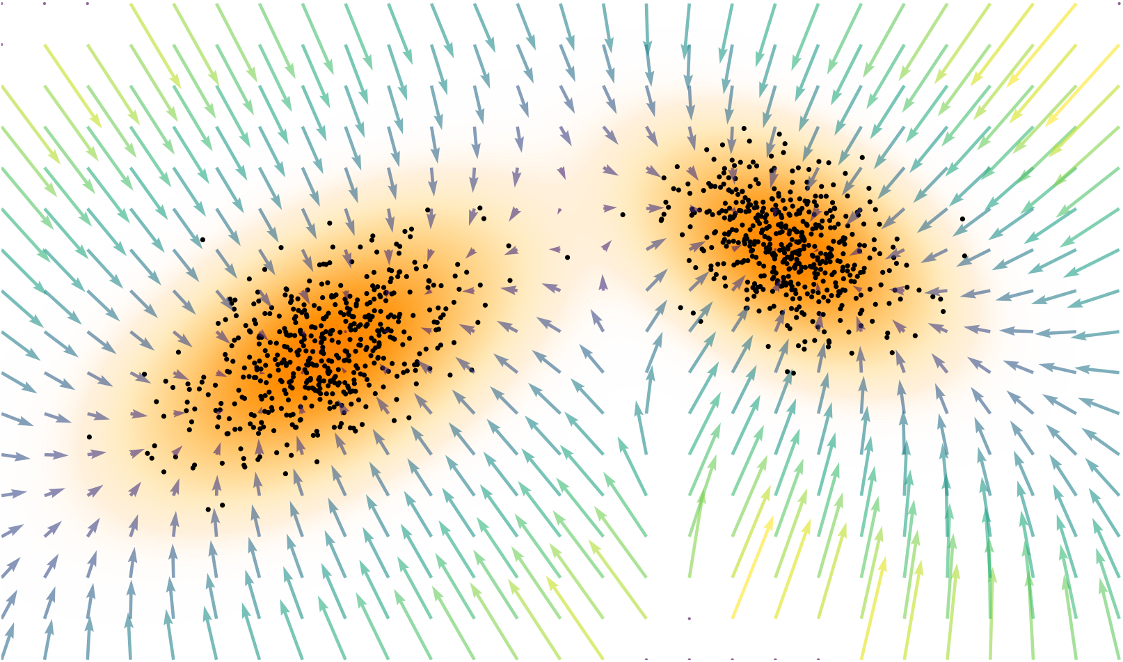
Score vector field points toward regions of higher data density.

Calculate the score function of EBM is irrelevant to the partition function:

And one can recover the density from the score function up to a constant:

Training EBM through Score Matching

And integration by parts gives an equivalent form that does not require : However, computing the Hessian trace is computationally expensive for high-dimensional data.

Langevin Sampling with Score Function

Without the partition function, we cannot directly sample from EBM. Instead, Langevin dynamics is used to generate samples.

Langevin Dynamics Sampling

Discrete-time Langevin dynamics: where is the step size.

Write in terms of score function:

Continuous-time Langevin dynamics: where is a Wiener process.

is used to ensure the stationary distribution is . This will be explained in the differential equation appendix.

The intution is that the score term pushes the sample toward high-density regions, while the noise term adds randomness to explore the space.

But Langevin dynamics is still struggling to sample from complex data distribution with many isolated modes, where it requires extremely long time to traverse low-density regions between modes.

3.2 From Energy-Based to Score-Based Generative Models

Once we have the score function, we can sample from the EBM using Langevin dynamics without computing the partition function. Therefore, we turn to directly learn the score function from data, leading to score-based generative models (SGMs).

The tractable score matching loss is

---

Proof of equivalence:

Focus on the second term:

The boundary term vanishes assuming decays to zero at infinity.

Note the third term is independent of , so we have the equivalence.

---

3.3 Denoising Score Matching

Although the tractable score matching loss avoids computing the partition function, it still requires calculating the Hessian trace , which is computationally expensive for high-dimensional data at complexity.

Sliced Score Matching

Let be an isotropic random vector, i.e., .

Then we have

So the score matching loss can be rewritten as

This can be computed using the Jacobian-vector product (JVP) technique, which only requires complexity.

Note the method only control the score function along random directions at observed data points, providing weak control in their neighborhood.

Denoising Score Matching (DSM)

Sliced score matching still need to compute the Jacobian-vector product. And the random directions introduce variance in optimization.

Vincent et al. (2011) proposed denoising score matching (DSM) to avoid computing the Hessian trace.

The idea is to add noise to data and learn the score function of the noisy data distribution.

This is equivalent to the denoising objective:

Under Gaussian noise corruption , we have .

The loss becomes

Tweedie’s Formula

Assume and .

Then we have: where the expectation is over the posterior distribution .

The proof is done by computing using Bayes’ theorem.

Higher cumulants of the posterior can also be computed through higher derivatives of .

Higher Order Tweedie’s Formula

Like , assume the conditional law of belongs to an exponential family with natural parameter :

For Gaussian noise with variance , , .

is the log-partition function of the .

The observed data distribution is

Define the log-partition function of as

Then the posterior of given is

By Bayes’ theorem,

The is the log-partition function of the posterior distribution.

For every , we have

Taking derivatives with respect to on both sides gives

Thus, we have Taking the second derivative gives

Higher order cumulants can be derived similarly by taking higher order derivatives of , which is a -th tensor for the -th cumulant.

Denoising, Tweedie and SURE

Stein’s Unbiased Risk Estimator (SURE) provides an unbiased estimate of the mean squared error (MSE) between a denoised estimate and the true signal without access to the true signal.

A denoiser is any weakly differentiable function that maps the noisy observation to a denoised estimate .

Quality of the denoiser is measured by the MSE:

The SURE states that the following quantity is an unbiased estimator of the MSE:

For the proof, first use the identity by integration by parts on each component.

Therefore

And then expand the MSE:

On the other hand Pointwise minimization of the MSE gives for almost every .

By Tweedie’s formula, we have

Therefore, we deduce

This shows the equivalence between denoising, score matching and SURE up to a constant depending on .

Generalized Score Matching

Omitted. TODO.

3.4 Noise Conditional Score Network (NCSN)